Introduction

\[\newcommand{\ds}{\displaystyle} \newcommand{\curlies}[1]{\left\lbrace #1 \right\rbrace} \newcommand{\abs}[1]{\left\lvert #1 \right\rvert} \newcommand{\angles}[1]{\left\langle #1 \right\rangle} \newcommand{\inv}[1]{#1^{-1}} \DeclareMathOperator{\supp}{supp} \DeclareMathOperator{\id}{id} \DeclareMathOperator{\rank}{rank} \DeclareMathOperator{\Mat}{Mat} \DeclareMathOperator{\Crit}{Crit} \newcommand{\A}{\mathcal A} \newcommand{\J}{\mathcal J} \newcommand{\RP}[1]{\R P^{#1}} \newcommand{\CP}[1]{\C P^{#1}} \newcommand{\bzero}{\mathbf 0} \newcommand{\a}{\mathbf a} \newcommand{\p}{\mathbf p} \newcommand{\u}{\mathbf u} \newcommand{\x}{\mathbf x} \newcommand{\y}{\mathbf y} \newcommand{\X}{\mathfrak X}\]

Intro to manifolds

The extrinsic perspective of an $n$-dimensional manifold is a subset of $\R^N$, usually as the level set of a function $\R^N \to \R^k$ where $n = N - k$. However, we will not adopt this perspective.

We will use the intrinsic definition, that an $n$-dimensional manifold is something that locally looks like $\R^n$.

The advantages of this are that:

• often there is no natural, unique, or canonical embedding of a manifold in $\R^N$
  • e.g. non-orientable surfaces cannot be embedded in $\R^3$
• extrinsic descriptions may be unnecessarily complicated
• a particular realization of a manifold as a subset of $\R^N$ is often irrelevant to questions that geometers ask

Some examples of manifolds are:

• The unit sphere in $\R^3$, i.e. the 2-sphere
• The set of all orthonormal bases of $\R^3$, which is homeomorphic to $SO(3)$
• the linkage of $N$ rods into a loop (this is only interesting for $N \geq 4$)
• the real projective plane $\RP2$, the set of all 1-dimensional subspaces (lines through the origin) in $\R^3$
  • $\RP2 = \curlies{x \in \R^3 : \abs x = 1}/\sim$ where $x \sim -x$

Coordinate charts

Coordinate charts

Let $M$ be a set. An $m$-dimensional coordinate chart $(U, \phi)$ is a subset $U \subseteq M$ and an injective map $\phi : U \to \R^m$ such that $\phi(U)$ is open. $U$ is called the chart domain and $\phi$ is called the coordinate map.

Two charts $(U, \phi)$ and $(V, \psi)$ are compatible if:

• $\phi(U \cap V)$ and $\psi(U \cap V)$ are open
• $\psi \circ \inv \phi : \phi(U \cap V) \to \psi(U \cap V)$ is a diffeomorphism

$\psi \circ \inv \phi$ is called a transition map or change of coordinates.

Compatibility of coordinate charts is not an equivalence relation, because it is not transitive.

Atlases

Let $M$ be a set. An $m$-dimensional atlas on $M$ is a collection of coordinate charts $\A = \curlies{(U_\alpha, \phi_\alpha)}_{\alpha \in A}$ such that:

• $\ds M = \bigcup_{\alpha \in A} U_\alpha$
• for all $\alpha, \beta \in A$, $(U_\alpha, \phi_\alpha)$ and $(U_\beta, \phi_\beta)$ are compatible

A coordinate chart $(U, \phi)$ is compatible with an atlas $\A$ if it is compatible with every chart in $\A$. Equivalently, $(U, \phi)$ is compatible with $\A$ if $A \cup \curlies{(U, \phi)}$ is still an atlas.

Compatible charts and atlases

Let $\A$ be an atlas on $M$, and let $(U, \phi)$ and $(V, \psi)$ be two charts on $M$. If $(U, \phi)$ and $(V, \psi)$ are both compatible with $\A$, then they are compatible with each other.

Consider $U \cap V$. Since they are coordinate charts on $M$ and the union of the domains of charts in $\A$ is $M$, we know that

\[U \cap V = \bigcup_{\alpha \in A} U \cap V \cap U_\alpha = \bigcup_{\alpha \in A} (U \cap U_\alpha) \cap (V \cap U_\alpha)\]

Since $U$ is compatible with every chart in $\A$, $U \cap U_\alpha$ is always open, and the same holds for $V$. Thus, $(U \cap U_\alpha) \cap (V \cap U_\alpha)$ is an open set for every $\alpha$, so each of these is open. An arbitrary union of open sets is open, so $U \cap V$ is open.

Maximal atlases

An atlas on $M$ is maximal if it is not a proper subset of a larger atlas, i.e. every chart that is compatible with $\A$ is already in $\A$.

Let $\A$ be an atlas on $M$, and let $\overline \A$ be the collection of all charts that are compatible with $\A$. Then $\overline \A$ is the unique maximal atlas containing $\A$.

Manifolds

First attempt at a definition

The following definition does not work:

An $m$-dimensional manifold is a set $M$ with a maximal $m$-dimensional atlas.

This definition has issues!

For example, with this definition, we can define some problematic “manifolds”:

• Let $M = \R$ and $\A = \curlies{(\curlies{\alpha}, \phi) : \alpha \in \R, \phi(x) = 0}$, so every $U_\alpha = \curlies \alpha$ and every $\phi_\alpha (x) = 0$. $\A$ is a maximal $0$-dimensional atlas, so this fits our definition.
  • We have shown $\R$ to be a 0-dimensional manifold. But this is not what we want - we’d like to think of $\R^1$ as a 1-dimensional manifold.
• Let $A = (-\infty, 0) \times \curlies 0$, $B^+ = \curlies{(t, t) : t > 0}$, and $B^- = \curlies{(t, -t) : t > 0}$, each is a subset of $\R^2$. Let $M = A \cup B^+ \cup B^-$. For our atlas, we can define […]
  • 
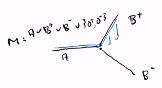
  • we do not want this to be a manifold

Definition of a manifold

An $m$-dimensional manifold is a set $M$ together with a maximal $m$-dimensional atlas $\A = \curlies{(U_\alpha, \phi_\alpha)}_{\alpha \in A}$ where:

• there are indices $\alpha_1, \alpha_2, …$ so that $\ds M = \bigcup_{i = 1}^\infty U_{\alpha_i}$ (countability)
• for any $p, q \in M$ where $p \neq q$, there are coordinate patches $U_\alpha$ and $U_\beta$ so that $p \in U_\alpha$, $q \in U_\beta$, and $U_\alpha \cap U_\beta = \emptyset$ (Hausdorff)

Hausdorff lemma

Let $M$ be a set with a maximal atlas $\A$. If $p, q \in M$ are points that are both in the domain $U$ of a single chart $(U, \phi) \in \A$, then the Hausdorff condition holds, i.e. there are disjoint coordinate patches $U_\alpha, U_\beta$ so that $p \in U_\alpha$ and $q \in U_\beta$.

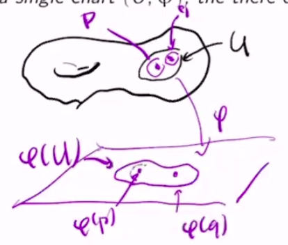
$\phi : U \to \R^m$ is injective, so $\phi(p) \neq \phi(q)$. Since $\R^m$ is Hausdorff, we can choose disjoint open sets $P, Q$ so that $\phi(p) \in P$ and $\phi(q) \in Q$. Let $U_\alpha = \inv\phi(P)$ and $U_\beta = \inv\phi(Q)$.

Examples of manifolds

• the $n$-sphere $S^n \subseteq \R^{n+1}$
• the real projective plane $\RP n = (\R^3 \setminus \curlies{0})/\sim$ where $\x \sim \y$ when there exists $\lambda \neq 0$ so that $\x = \lambda \y$
  • note that $\RP n = \R^n \sqcup \R^{n-1} \sqcup … \sqcup \R^1 \sqcup \R^0$
• the real Grassmanian

The real Grassmanians

The real Grassmanian, $Gr(k, n)$, is the set of all $k$-dimensional subspaces of $\R^n$. It is a manifold of dimension $n-k$.

Note that $Gr(1, n) = \RP {n-1}$.

Suppose $I \subseteq \curlies{1, …, n}$, then we use the notation $I’$ to denote $I’ = \curlies{1, …, n} \setminus I$. Assume from here on that $\abs I = k$.

We use this notation to denote subspaces of $\R^n$ generated by the directions in $I$, so

\[\R^I = \curlies{\x \in \R^n : x^i = 0 \text{ whenever } i \in I'}\]

It is clear that $\R^I \in Gr(k, n)$. Also note that $\R^{I’} = (\R^I)^\perp$.

Subspaces that intersect $\R^{I’}$ trivially

Define the set

\[U_I = \curlies{E \in Gr(k, n) : E \cap \R^{I'} = \curlies 0}\]

i.e. the set of $k$-dimensional subspaces of $\R^n$ that intersect trivially with $\R^{I’}$. If $E \in U_I$, then there is a unique linear map $A_I : \R^I \to \R^{I’}$ so that

\[E = \curlies{y + A_I(y) : y \in \R^I}\]

To prove this, define $\pi_I : \R^n \to \R^I$ and $\pi_{I’} : \R^n \to \R^{I’}$ as projections into their respective subspaces.

Consider $\widetilde \pi_I = \pi_I \vert_E : E \to \R^I$. Suppose $x \in E$ and $\pi_I (x) = 0$, then

\[\begin{align*} x &= \pi_I(x) + \pi_{I'}(x) \\ x &= \pi_{I'}(x) \end{align*}\]

so $x \in \R^{I’}$, i.e. $x \in E \cap \R^{I’} = \curlies 0$, so $x = 0$. Thus, $\widetilde \pi_I$ is injective. Its domain $E$ has dimension $k$, so its range does as well. However, its codomain is $\R^I$ which has dimension $k$ as well, so $\widetilde \pi_I $ is an isomorphism.

Define $A_I = \pi_I’ \circ \inv{\widetilde \pi_I}$. If $y \in E$, then

\[\begin{align*} x &= \pi_I(x) + \pi_{I'}(x) \\ &= x + \pi_{I'} \circ \inv{\widetilde \pi_I} \circ \widetilde \pi_I (x) \\ &= x + \pi_{I'} \circ \inv{\widetilde \pi_I} (x) \tag{since $x \in E$} \\ &= x + A_I(x) \end{align*}\]

so in conclusion,

\[E = \curlies{x + A_I(x) : x \in \R^I} = \begin{pmatrix} \id_k \\ A_I \end{pmatrix} \R^I\]

If $L(\R^I, \R^{I’})$ is the set of linear maps from $\R^I$ to $\R^{I’}$, then the work above gives us a bijection between elements of $Gr(k, n)$ and $L(\R^I, \R^{I’})$. Each linear map in $L(\R^I, \R^{I’})$ corresponds to a unique matrix in $\Mat_\R((n-k) \times k)$, so we now have a bijection

\[\begin{align*} \phi : U_I &\to \Mat_\R((n-k) \times k) \\ E &\mapsto A_I \end{align*}\]

$\Mat_\R((n-k) \times k) \cong \R^{(n-k) \times k}$, so we can consider the pair $(U, \phi)$ to be a chart for $Gr(k, n)$.

[…]